Numerical Tests

In numerical simulations we considered two types of dispersal kernels in (4): the Gaussian kernel,

$$K(x)=\frac{1}{\sigma \sqrt{2\pi}}\, e^{-\frac{x^2}{2\, \sigma^2}},$$ (24)

and the Laplace kernel

$$K(x)=\frac{1}{2\, \sigma}\, e^{-\frac{\vert x\vert}{\sigma}},$$ (25)

where $\sigma$ is the mean distance traveled by spores in meters (nominally set to 1 meter). These two kernels are among the most commonly used for dispersal studies. The Guassian form describes a process of random dispersion in the horizontal direction as spores fall from a given height to the ground; the Laplace kernel describes the net results of a random horizontal diffusion in time coupled with a constant rate of precipitation of spores to the ground. Convolution and dispersal were implemented using Fast Fourier Transforms and the property that the transform of the convolution is the product of the transforms. In all simulations 4096 grid points were used; the size of the spatial domain was $180 \times v^*$ meters, where $v^*$ is the maximum predicted velocity. Given initial conditions starting in the center of the domain, this gave enough space so that in 60 `days' of simulation a developing front had 1.5 times as much room to propagate as the maximum speed linear prediction. Boundary conditions were taken to be periodic.

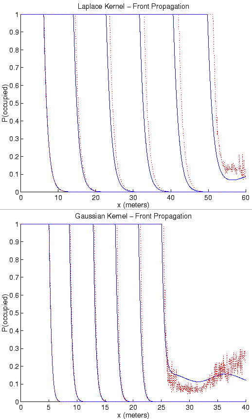
Figure 4: Evolution of the front from initial conditions $N_1^0 = 10^4, \vert x\vert<3, N_*^0 =0$ otherwise, in the case of the Laplace kernel (top) and Gauss kernel (bottom), with nominal parameters as given in Table 1. The fraction of resource occupied, $1-P_{\mbox{\tiny unocc}}$, is plotted here. Time slices are ten days apart, with the evolution of the nonlinear front given by solid lines and the linear front given by dotted line. Notice that during the last time slice small round-off errors have grown in advance of the front; these eventually grow and dominate the solution. The nonlinear solution looks much smoother at this point because calculation of $P_{\mbox{\tiny unocc}}$ involves summing over age classes, which smooths the instability.

Each simulation was performed in the non-linear case using (2), where $P_{\mbox{\tiny unocc}}$ from (3) was recomputed in each step (each day) using formula (1), and in the linearized case using (6). The behavior of $P_{\mbox{\tiny unocc}}$ and shape of typical fronts for parameters as in Table 1 and both Laplace and Gaussian kernels is depicted in Figure 4, for both linear and nonlinear growth rates. In both cases, $P_{\mbox{\tiny unocc}}$ was used to diagnose and depict the location of the front; that is, to determine the location of the wave of invasion each `day' we would calculate $P_{\mbox{\tiny unocc}}$ (even if it was not used in the dynamics, as in the linear simulations) and determine the current extent of the invasion by determining which grid cell contained that point where $P_{\mbox{\tiny unocc}}= \frac12$. From the obtained results we then deduced the speeds of invasion ( $v_{\mbox{\tiny non-linear}}$ and $v_{\mbox{\tiny linearized}}$, respectively) in both non-linear and linear settings by calculating the distances propagated over 10 days at the end of the simulation.

For each simulation we also computed the upper bound of the invasion speed $v^*$ from (10) as follows: we multiplied the composite constant $R$ from (5) and the moment generating function $M(s)$ from (8) to obtain $\rho$ from (18). This $\rho$ was then inserted into (23) to obtain $\lambda _1(s)$. Finally, $\lambda _1(s)$ was inserted into (10), and the minimum over $s$ was computed, giving $v^*$. The speed of invasion $v^*$ should match the speed obtained by the simulation in the linearized case. According to (8), the moment generating function is given by

$$M(s)=e^{\frac{\sigma^2 s^2}{2}}$$

for the Gaussian kernel (24), and by

$$M(s)=\frac{1}{1-\sigma^2 s^2},$$

for the Laplace kernel (25).

Figure: Progress of an invasion with mean spore dispersal distances of 1 meter using Gaussian (left) and Laplace (right) kernels. Parameters are set to nominal values described in Table 1. Invasions were allowed to progress linearly (unoccupied resource fraction, $P_{\mbox{\tiny unocc}}$, set always to 1, dashed lines) and nonlinearly (solid lines). The predicted speeds are $v^*=0.415$ meters/day for the Gaussian kernel and $v^*=0.936$ meters/day for the Laplace kernel, which is a small overestimate of the linear propagation speeds and a larger overestimate of the nonlinear speeds.

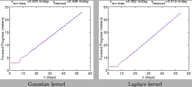Figure 5 shows an example of simulation with nominal values of parameters from Table 1. For these values, the composite constant $R$ from (5) and (17) is equal to $R=10.0531$. The simulation was run with Gaussian and Laplace kernel, respectively, with $\sigma=1$ in both cases. Solid curves show the progress of infection in the non-linear cases, and dashed curves show the progress in the linearized cases with $P_{\mbox{\tiny unocc}}=1$ in (3). For this example the theoretical speeds are $v^*=0.415$ meters/day for the Gaussian kernel and $v^*=0.936$ meters/day for the Laplace kernel. We see that, for both kernels, the speeds obtained by linearization, $v_{\mbox{\tiny linearized}}$, overestimate the speeds of the nonlinear model, $v_{\mbox{\tiny non-linear}}$, and the theoretical speeds $v^*$ slightly overestimate $v_{\mbox{\tiny linearized}}$. This is quite interesting, as the dynamic perspective on front propagation would suggest that $v^*$ should be the asymptotic speed for both linear and nonlinear fronts, and simulation result with fixed-size Leslie matrices indicate rapid convergence to the predicted minimal wave speed (see, for example, Neubert and Caswell [15]).

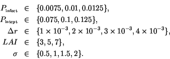
To more completely investigate the comparative behavior of $v_{\mbox{\tiny non-linear}}$ versus $v^*$ and $v_{\mbox{\tiny linearized}}$ versus $v^*$, we performed a series of simulations with different values of parameters from Table 1 in a randomized factorial design. The first three parameters ($SI$, $LP$ and $IP$) were kept at their nominal values, while the remaining five parameters were chosen as follows:

$$\begin{eqnarray*} P_{\mbox{\tiny infect}}&\in& \{ 0.0075, 0.01, 0.0125\},\\ P_{... ...,\\ LAI &\in& \{ 3,5,7\}, \\ \sigma &\in& \{ 0.5, 1, 1.5, 2\}. \end{eqnarray*}$$

This gives the total of 432 simulations for each kernel. In these simulations, the composite constant $R$ attained values in the interval $R\in[0.3534,15.7080]$, and the theoretical bound for invasion speed $v^*$ attained values $v^*\in[0.1198,0.8755]$ for the Gaussian kernel and $v^*\in[0.2376,2.0106]$ for the Laplace kernel. The results of simulations are summarized in Figure 6.

Figure 6: Comparison of predicted and observed speeds for waves of invasion with and without density dependent growth restrictions for both Laplace and Gaussian dispersal kernels. Parameters are chosen in a random factorial design described in the text, with variation centered on the nominal values described in Table 1. Observed linear and nonlinear speeds are marked with `$\circ$' and `*' respectively. The solid line is the line $v_{\mbox{\tiny observed}}= v_{\mbox{\tiny predicted}}$, indicating perfect agreement. Results indicate a consistent overprediction of observation by prediction, with a greater degree of error for nonlinear as compared to linear propagation.

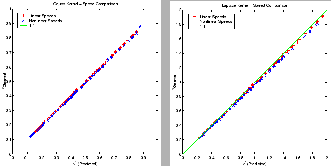The size of the error between observation and prediction depicted in Figure 6 reflects what appears to be a consistent overprediction of observed linear and nonlinear speeds, with the degree of overprediction being approximately double for nonlinear speeds as compared to linear speeds. From the minimal speed perspective this is not so awful; after all, $v^*$ is an upper bound, but only in relatively rare cases has it been proven to be the asymptotic speed of fronts. On the other hand, the agreement between prediction and observation is generally superb (see, for example, Neubert et al. [15,16])- why should it be less so in this case? And what of the dynamic argument, which suggests that fronts should accelerate to $v^*$?

The explanation for the degree of observation lies in three interrelated effects in our simulation. In the first place, the net daily per-capita growth rate for the number of fungal lesions was never less than 1.5 in our simulations, and was often as large as 10, reflecting the extremely invasive nature of this pathogen. As a consequence, simulations were difficult to run for long periods of time; at some point small round-off errors in the neighborhood of zero would start to grow geometrically. So, in practice we were unable to maintain simulations much beyond 50 iterations, and running longer simulations to allow for greater convergence was impossible both because of the extreme instability of the zero population state as well as the size of the transition matrices (which are as large as the number of days) at each spatial location.

Confounded with this effect are two convergence effects, each contributing to the overprediction. In the first place there is the convergence to the stable travelling population distribution, which is described by the first neglected terms in the power method. Thus, when considering the evolution of a front from compact initial data, the asymptotic problem should read

$$\begin{eqnarray*} e^{ns^*v^*} \ \vec{w} = \textbf{H}^n (s^*) \ \vec{w} &=& a_1(... ...rac{\lambda_2^n}{\lambda_1^n} \vec{e}_2(s^*) + \cdots \right]. \end{eqnarray*}$$

Here $\vec{e}_1(s^*)$ can be interpreted as the asymptotic stable population distribution selected by the wave of invasion, while $\vec{e}_2(s^*)$ is the age structure of the `ringing' which occurs as population distributions converge to the stable distribution along a front, and the ratio of the largest and second-largest magnitude eigenvalues is the rate of convergence. This is asymptotically negligible, but for finite duration simulations (like those we are forced to run by the extreme instability of the system) we may expect an error in estimating front speeds proportional to

$$E_{\mbox{\tiny Power}} \sim \vert\vec{e}_1 \cdot \vec{e}_2\vert \frac{\vert\lambda_2\vert^n}{\vert\lambda_1\vert^n} .$$ (26)

The second convergence effect is the natural acceleration of the front to the asymptotic front speed described by (16). Predicted by the steepest descent methodology, this can be viewed as the convergence of the spatial shape of the front to the asymptotic exponential shape which is a translate of $e^{-s^* x}$. The speed convergence error predicted by the steepest descents approach is (from 16)

$$E_{\mbox{\tiny Speed}} \sim \frac{\ln(n)}{2 n k^*}.$$ (27)

While $E_{\mbox{\tiny Speed}}$ tends to zero as $n$ tends to infinity, the convergence is slow, and again the constraint that we were unable to simulate for more than several tens of iterations means that this error can not be neglected.

To investigate how these errors relate to observed errors in our simulation we ran each of the factorially crossed parameter studies for as long as possible, diagnosing the onset of overwhelming instability by the inevitable sudden jump in the rate of progress of the front. In each simulation the day at which the simulation `broke' was diagnosed by and recorded as $nday$. During each simulation the forward progress ($x_{fp}$) of the front was diagnosed as described above. Observed speeds were then diagnosed by

$$v_{\mbox{\tiny observed}} = \frac{x_{fp}(nday-5)-x_{fp}(nday-15)}{10}.$$

Simultaneously, the largest two eigenvalues of the finite transition matrix, $\lambda_1^{m}(s^*)$ and $\lambda_2^{m}(s^*)$, were calculated, with $m$ evaluated at the center of the speed calculation interval, $m=nday-10$. With this information we could determine the size of the two error components, $E_{\mbox{\tiny Power}}$ and $E_{\mbox{\tiny Speed}}$. These errors are compared to the observed relative speed error,

$$\frac{v^*-v_{\mbox{\tiny observed}}}{v^*},$$

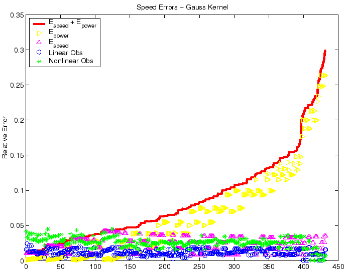
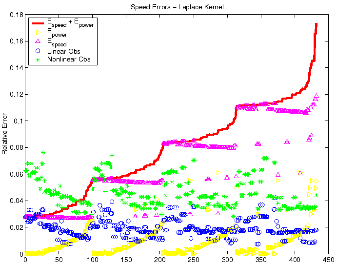
in Figures 7 and 8.

Figure 7: Raw comparison of observed relative speed errors in the nonlinear (`*') and linear (`$\circ$') cases for the Gaussian kernel, with randomized choices of parametric data, centered on the nominal values in Table 1. The asymptotic error size due to age structure convergence, $E_{\mbox{\tiny Power}}$, is plotted as ` $\triangleright$', while asymptotic error size due to speed convergence, $E_{\mbox{\tiny Speed}}$, appears as `$\triangle$'. The total error size, $E_{\mbox{\tiny Speed}}+E_{\mbox{\tiny Power}}$ is the solid line; results were sorted in terms of increasing total error. The horizontal axis is the identifying index of the simulation and has no units. Given that the actual error relates by an order one factor to the error sizes depicted here, both the linear and nonlinear front speeds are well within acceptable error bounds.

Figure 8: Raw comparison of observed relative speed errors in the nonlinear (`*') and linear (`$\circ$') cases for the Laplace kernel, with randomized choices of parametric data, centered on the nominal values in Table 1. The asymptotic error size due to age structure convergence, $E_{\mbox{\tiny Power}}$, is plotted as ` $\triangleright$', while asymptotic error size due to speed convergence, $E_{\mbox{\tiny Speed}}$, appears as `$\triangle$'. The total error size, $E_{\mbox{\tiny Speed}}+E_{\mbox{\tiny Power}}$ is the solid line; results were sorted in terms of increasing total error. The horizontal axis is the identifying index of the simulation and has no units. Given that the actual error relates by an order one factor to the error sizes depicted here, both the linear and nonlinear front speeds are well within acceptable error bounds.